Sentiment Analysis of Anne of Green Gables

Anne of Green Gables is probably the best known novel by Canadian author Lucy Maude Montgomery. The series of eight novels, of which Anne of Green Gables is the first, revolves around Anne Shirley and her life from age 11 until the end of the first world war, when she is 40 years old. I enjoy almost all of Montgomery’s books so I thought it would be interesting to take a closer look at her work using some natural language processing techniques, specifically sentiment analysis.

Natural Language Processing

So, what is natural language processing (NLP)? Basically, it is the process of using computers to analyze and extract information from natural (human) language. NLP is field of study that overlaps with computer science, artificial intelligence, and computational linguistics. Some of the more common or familiar tasks in NLP include: machine translation, automatic summarization, speech recognition, parsing (analyze grammar), and sentiment analysis.

Sentiment analysis is used to quantify the emotional state or attitude of a speaker or writer. This is usually determined by measuring the polarity of the words in the text: are they positive, negative, or neutral? A sentiment polarity value can be determined for an individual word, a complete sentence, or an arbitrary chunk of text such as a tweet or movie review.

This sentiment analysis of Anne of Green Gables will focus on how the relative sentiment polarity changes over the course of the novel. Eventually, I would like to analyze the sentiment for each of the novels in the Anne series and compare with the sentiment of the novels in the Emily series. In order to analyze the novel, we need the next! Almost all of Montgomery’s work is available at Project Gutenberg.

# Import this stuff to make Python 3 functions work in Python 2
from __future__ import division
from __future__ import print_function

from urllib2 import urlopen
from unidecode import unidecode

url = "http://www.gutenberg.org/files/45/45-0.txt" # text for "Anne of Green Gables"
response = urlopen(url)
raw = response.read().decode('utf8') # Convert bytes to unicode
raw_decode = unidecode(raw) # Decode some "weird" characters to the closest ascii equivalent
raw_string = str(raw_decode) # Convert from unicode string to plain string
raw_string = raw_string.replace('\r\n', ' ') # replace the " \r\n " characters with a space

Now we have the text of the novel, including the header and footer information from Project Gutenberg. The text is currently a single string of characters, including punctuation and spaces. The header (and the list of chapters) and the standard footer will be sliced out to end up with just the body of the novel.

# Remove the header, footer, and chapter list
start = raw_string.find("MRS. Rachel Lynde lived just where the Avonlea")
stop = raw_string.find("End of Project Gutenberg's")
raw_string = raw_string[start:stop]

Tokenization

Because the text is a single long string of characters, it needs to be tokenized or broken down into smaller pieces of text. In natural language processing, tokens are usually words or sentences. I will be using the VADER analysis tool, which was designed to classify the sentiment of text at the sentence level, so that’s what we’ll do. We’ll take a closer look at VADER in a minute but first the text needs to be parsed into sentences.

If you are using python for NLP tasks, you are probably going to be using the Natural Language Tool Kit (NLTK). Let’s tokenize and then take a look at some of the sentences to make sure the string was broken down correctly. You will need to have installed the NLTK from the above link before importing the modules.

# Import the the NLTK package and the sentence tokenizer function
import nltk
from nltk import sent_tokenize

# Tokenize into sentences
sentences = sent_tokenize(raw_string)
print("Number of sentences in the novel:", len(sentences))

Number of sentences in the novel: 6855

Let’s look at a section of the novel to check the tokenization. How about the part where Anne describes the poor mouse who met an untimely end in the pudding sauce?

# Find the sentence index for the pudding sauce sentence
sauce = sentences.index("She was terribly mortified about the pudding sauce last week.")

for i in range(sauce,sauce+8):
    print(i, sentences[i])

2904 She was terribly mortified about the pudding sauce last week.
2905 We had a plum pudding for dinner on Tuesday and there was half the pudding and a pitcherful of sauce left over.
2906 Marilla said there was enough for another dinner and told me to set it on the pantry shelf and cover it.
2907 I meant to cover it just as much as could be, Diana, but when I carried it in I was imagining I was a nun - of course I'm a Protestant but I imagined I was a Catholic--taking the veil to bury a broken heart in cloistered seclusion; and I forgot all about covering the pudding sauce.
2908 I thought of it next morning and ran to the pantry.
2909 Diana, fancy if you can my extreme horror at finding a mouse drowned in that pudding sauce!
2910 I lifted the mouse out with a spoon and threw it out in the yard and then I washed the spoon in three waters.
2911 Marilla was out milking and I fully intended to ask her when she came in if I wouldd give the sauce to the pigs; but when she did come in I was imagining that I was a frost fairy going through the woods turning the trees red and yellow, whichever they wanted to be, so I never thought about the pudding sauce again and Marilla sent me out to pick apples.

Those sentences look good; there is a mix of longer and shorter sentences in addition to some dialogue that is correctly tokenized. Let’s take a look at the sentiment polarity for each sentence. To do this, we finally get to talk about VADER. VADER stands for “Valence Aware Dictionary for sEntiment Reasoning” and is a rule-based lexicon for evaluating sentiment polarity (positive or negative).

Valence refers to verb valency or how a verb relates to the arguments in a sentence. The sentiment of some words or phrases in a sentence can be changed by other words present in the sentence. The words that modify the sentiment can be called valence-shifters. Examples of these are negatives (not, never), intensifiers (very, really), diminishers (a bit, slightly), and connectors (however, but, although). There is a lot more that could be said about VADER but I will leave that for another notebook.

Let’s look at a few sentences individually to see what sort of scores are returned from VADER. Since we already have part of the pudding sauce story printed above, we’ll use a couple of those sentences. You will need to install the VADER library before using the sentiment tools.

# The following is to fix a problem of printing to the console after VADER is imported.
# The system standard output variables are saved in nb_stdout and then reset after importing VADER
# (fix from: https://github.com/cjhutto/vaderSentiment/issues/7)

import sys
nb_stdout = sys.stdout
from vaderSentiment.vaderSentiment import sentiment as vaderSentiment
sys.stdout = nb_stdout

for i in [2886,2904,2908,2909]:
    print(sentences[i])
    vs = vaderSentiment(sentences[i])
    print("\n\t" + str(vs) + "\n\n")

The tumblerfuls were generous ones and the raspberry cordial was certainly very nice.

    {'neg': 0.0, 'neu': 0.532, 'pos': 0.468, 'compound': 0.8313}


She was terribly mortified about the pudding sauce last week.

    {'neg': 0.286, 'neu': 0.714, 'pos': 0.0, 'compound': -0.5574}


I thought of it next morning and ran to the pantry.

    {'neg': 0.0, 'neu': 1.0, 'pos': 0.0, 'compound': 0.0}


Diana, fancy if you can my extreme horror at finding a mouse drowned in that pudding sauce!

    {'neg': 0.36, 'neu': 0.64, 'pos': 0.0, 'compound': -0.8356}

Sentiment Polarity

VADER returns the values for negative, neutral, positive, and compound. The compound is the overall polarity of the sentence, given as a number between -1 and 1. The higher the compound score, the more positive the sentiment of the sentence. The first sentence is quite positive but the second and last sentences are definitely more negative. The third sentence is pretty neutral, with a compound score of 0 since there are neither positive or negative words.

Now that we have a better idea of what a sentiment value for different types of sentences looks like, we will go ahead and find the sentiment for all of the sentences in the novel. A definite advantage of VADER is that it is efficient (for a python program) and does not take very long at all to go through the entire novel (just a few seconds on my old-ish laptop running linux).

# Determine the score of each sentence and make a list of just the compound or polarity values
complete_score = [vaderSentiment(sentence) for sentence in sentences]
polarity = [line.get('compound') for line in complete_score]

# Import the modules needed to use matplotlib and have the plots inline in the notebook
%matplotlib inline

import matplotlib
import numpy as np
import matplotlib.pyplot as plt
from pylab import rcParams

# Plot the polarity of the sentiment as a function of sentence number in the text.
rcParams['figure.figsize'] = 14, 4
plt.plot(polarity,'b.')
plt.xlabel('Sentence Index'), plt.ylabel('Sentiment Polarity')
plt.axis([0, len(sentences), -1.10, 1.10])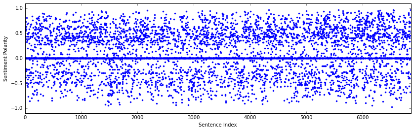

That is a lot of sentences and sentiment values! It is difficult to see any patterns in the sentiment other than that is is more positive than negative and there are a number of neutral sentences (polarity = 0). In order to better visualize any changes, it would be helpful to apply a running average over a window of an appropriate width, the width being the number of sentences averaged together. If the window is too large, some of the changes in sentiment will be averaged away and changes on shorter “time” scales might be lost.

To determine a good window width, we can calculate the averaged sentiment for a number of different window sizes and visually determine what looks to be the best. This is still going to be somewhat subjective in terms of what any given individual would deem “too smooth” or “too noisy”. And of course, it would depend on the novel. A really long novel with a slowly unfolding plot would probably do okay with averaging over a large window; a fast-paced or shorter book might do better with a smaller number of sentences averaged together.

First, we’ll define a function to calculate the running average.

# Define a running mean function that averages over a given window of width N (width = number of sentences)
def running_mean(x, N):
    run_sum = np.cumsum(np.insert(x,0,0))
    return(run_sum[N:]-run_sum[:-N])/N


# Calculate a new list (vector) of polarity values, averaged over the window 
# values of N between 50-80 sentences gave good results
polarity_ave = running_mean(polarity, 60)

# Create a vector of values for the x-axis as a percentage of the novel
xvalues = [index*100/len(polarity_ave) for index in range(len(polarity_ave))]

# Calculate another vectory of polarity values with a very small window (to compare later in a plot)
polarity_ave_small = running_mean(polarity, 5)

# Create a vector of values for the x-axis as a percentage of the novel
xvalues_small = [index*100/len(polarity_ave_small) for index in range(len(polarity_ave_small))]

rcParams['figure.figsize'] = 14, 6

plt.subplot(211)
plt.subplots_adjust(wspace=0.5, hspace=0.75);
plt.plot(xvalues_small, polarity_ave_small, 'g-', alpha=0.5)
plt.fill_between(xvalues_small, 0, polarity_ave_small, facecolor='green', alpha=0.5)
plt.axis([0, 100, -0.75, 0.75])
plt.axhline(y=0, xmin=0, xmax=100)
plt.ylabel('Sentiment Polarity')
plt.title('Running Average with N = 5')

plt.subplot(212)
plt.plot(xvalues, polarity_ave, 'g-', alpha=0.5)
plt.fill_between(xvalues, 0, polarity_ave, facecolor='green', alpha=0.5)
plt.axis([0, 100, -0.75, 0.75])
plt.axhline(y=0, xmin=0, xmax=100)
plt.xlabel('Percent of Novel'), plt.ylabel('Sentiment Polarity (averaged)')
plt.title('Running Average with N = 60')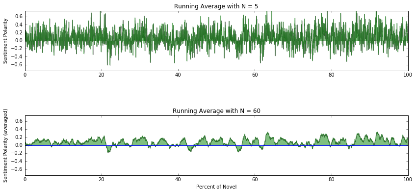

The top plot is using a running average with a small window (averaging over a small number of sentences) and is essentially the “raw” sentiment of the novel, showing how sentiment changes over short time scales. There are a lot of positive and negative spikes but we can start to see a little bit of a pattern when looking at the lower frequencies or longer time scales.

The bottom plot with with a running average window of 60 sentences and it is now much easier to see changes in sentiment that happen over longer time intervals. There are definite high and low periods that were not averaged away. The magnitude of the sentiment decreased because of the averaging but since we are looking at relative changes over the course of the novel, the absolute scale shouldn’t matter.

To take a closer look at events in the novel, we’ll split the novel in half and plot each part separately. We can also annotate the plot with what is happening in the novel. Because you were dying to know what all the positive and negative parts were, right?

# Make a string with the anne-otations to be added to the plot below
text = ['Anne is not a boy','Anne yells at Mrs. Lynde','Anne meets Diana','Diana gets drunk','No more Diana!']
text.extend(['Haunted woods & Mr. Phillips departs','Anne\'s Broken ankle','Miss Stacey!','Charlottetown trip'])
text.extend(['Miss Stacey leaves','Anne wins the Avery'])

# Make more strings with the position of the text and arrows
xy_pos = [(7.3,-0.08),(22.5,-0.18),(28.44,0.25),(42.28,0.25),(43.5,-0.175)]
xytext_pos = [(6.8,-0.2),(24,-0.25),(24,0.4),(43,0.4),(44,-0.25)]

xy_pos.extend([(55.7,-0.18),(61.75,-0.12),(63.4,0.375),(77,0.3),(84.33,-0.13),(92.79,0.3)])
xytext_pos.extend([(56.5,-0.25),(62,-0.25),(64.75,0.4),(73,0.4),(81,-0.25),(93,0.45)])

rcParams['figure.figsize'] = 16, 8

plt.subplot(211)
plt.plot(xvalues, polarity_ave, 'g-', alpha=0.5)
plt.fill_between(xvalues, 0, polarity_ave, facecolor='green', alpha=0.5)
plt.axis([0, 50, -0.3, 0.5])
plt.axhline(y=0, xmin=0, xmax=50)
plt.ylabel('Sentiment Polarity (averaged)')
plt.title('Running Average with N = 60')

for i in range(0,5):
    plt.annotate(text[i], xy=xy_pos[i], xytext=xytext_pos[i], arrowprops={'arrowstyle': '-'}, va='center')

plt.subplot(212)
plt.plot(xvalues, polarity_ave, 'g-', alpha=0.5)
plt.fill_between(xvalues, 0, polarity_ave, facecolor='green', alpha=0.5)
plt.xlabel('Percent of Novel'),plt.ylabel('Sentiment Polarity (averaged)')
plt.axis([50, 100, -0.3, 0.5])
plt.axhline(y=0, xmin=50, xmax=100)

for i in range(6,11):
    plt.annotate(text[i], xy=xy_pos[i], xytext=xytext_pos[i], arrowprops={'arrowstyle': '-'}, va='center')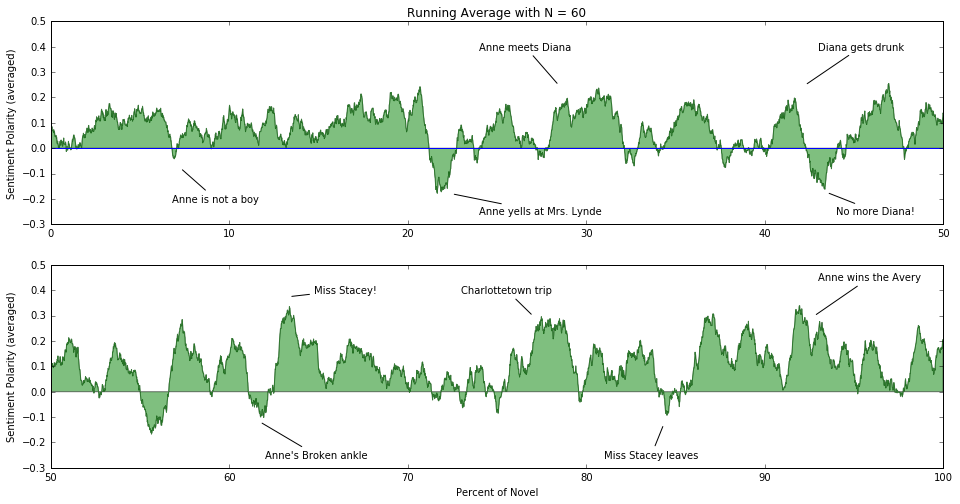

The parts of the novel that a reader would likely identify as positive (new best friend, lovely new teacher, winning a scholarship) are the parts with the highest sentiment polarity. And the parts of the novel that are more negative (yelling at someone, missing a best friend, injury, and sickness) are t!e sections with the most negative sentiment. It looks like VADER did a pretty good job with this text.

Let’s take a look at another sentiment classifier and how the results compare to VADER. There is a handy text processing library called TextBlob that makes it much easier to implement many of the functions available in the NLTK. The default sentiment classifier used by TextBlob is the PatternAnalyzer. The TextBlob module needs to be installed before you can use the functions.

# TextBlob
from textblob import TextBlob

# Use the TextBlob to tokenize the raw string and make a textblob object
anne_blob = TextBlob(raw_string)

# Determine the sentiment using the PatternAnalyzer (based on the pattern library)
blob_sentiment = [sentence.sentiment.polarity for sentence in anne_blob.sentences]

And then we can plot the sentiment as a function of sentence index.

# Plot the polarity of the sentiment as a function of sentence number in the text.
rcParams['figure.figsize'] = 14, 4
plt.plot(blob_sentiment,'b.')
plt.xlabel('Sentence Index'), plt.ylabel('Sentiment Polarity')
xmax = len(blob_sentiment)
plt.axis([0, xmax, -1.10, 1.10])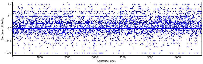

The sentiment values from the PatternAnalyzer classifier looks similar to those determined by VADER. The sentiment is overall more positive than negative and tends toward more positive values near the end of novel. The polarity values also tend to cluster at 0.5, 1.0, and -1.0; I’m not quite sure what is causing that.

In order to better compare the two sentiment classifiers, I’ll make another plot. But first, the TextBlob sentiment also needs to be averaged using the same method applied to the VADER sentiment values. Then come the plots!

# Calculate a new list (vector) of polarity values, averaged over the window N = 60
blob_ave = running_mean(blob_sentiment, 60)

# Create a vector of values for the x-axis as a percentage of the novel
xvalues_blob = [index*100/len(blob_ave) for index in range(len(blob_ave))]

# Plot the sentiment for each classifier
rcParams['figure.figsize'] = 16, 8

plt.subplot(211)
plt.plot(xvalues, polarity_ave, 'g-', alpha=0.5)
plt.fill_between(xvalues, 0, polarity_ave, facecolor='green', alpha=0.5)
plt.axis([0, 100, -0.3, 0.4])
plt.axhline(y=0, xmin=0, xmax=100)
plt.ylabel('Sentiment Polarity (averaged)')
plt.title('VADER Sentiment (running average window = 60)')

plt.subplot(212)
plt.plot(xvalues_blob, blob_ave, 'g-', alpha=0.5)
plt.fill_between(xvalues_blob, 0, blob_ave, facecolor='green', alpha=0.5)
plt.xlabel('Percent of Novel'),plt.ylabel('Sentiment Polarity (averaged)')
plt.axis([0, 100, -0.3, 0.4])
plt.axhline(y=0, xmin=0, xmax=100)
plt.title('TextBlob/Pattern Sentiment (running average window = 60)')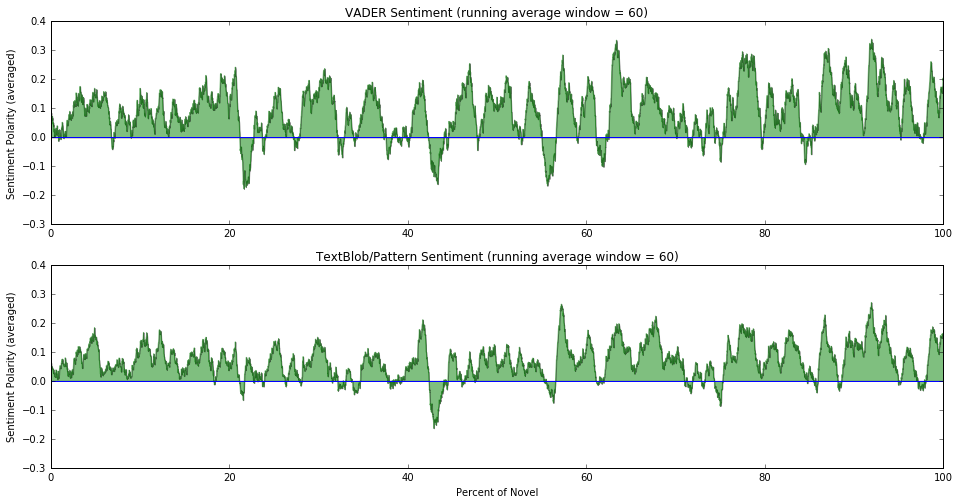

The results look reasonably similar but there are some notable differences. First, using VADER, there is a big dip into negative sentiments when Anne yells at Mrs. Lynde - that is the first time that anything really negative happens in the novel. The PatternAnalyzer almost completely misses it, with only a small dip in sentiment about a quarter of the way through the novel. In general, VADER picks up more negative sentiment overall than PatternAnalyzer. This would certainly be something to examine further.

There are many other interesting things to analyze: sentence length, word length, word frequency, and other sentiment classifiers. We’ll look at just a couple of them now. First, let’s take a look at a histogram of sentence length, as determined by the number of characters in a sentence. These types of histograms would be interesting to compare for the rest of the books in the Anne series in addition to the other work by Montgomery. Using sentences of different lengths adds variety and interest to a piece of writing and different authors have different distributions of sentence length.

# Make a histogram of sentence lengths (in this case, the number of characters per sentence)
sen_length = [len(sentence) for sentence in sentences]

plt.hist(sen_length, bins=150)
plt.ylabel('Number'), plt.xlabel('Sentence Length (characters)')
plt.title('Anne of Green Gables')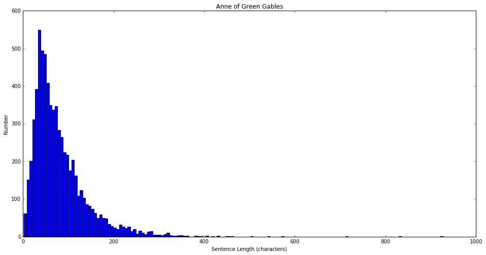

We can also look at how sentence length compares to the sentiment. Do longer sentences tend to be positive or negative? Will there be any correlation at all between sentence length and sentiment? Let’s find out.

# Plot the sentiment score as a function of sentence length

plt.plot(sen_length, polarity,'b.')
plt.axis([0, 450, -1.0, 1.0])
plt.xlabel('Sentence Length (number of characters)')
plt.ylabel('Sentiment Polarity')
plt.title('Sentiment as a Function of Sentence Length')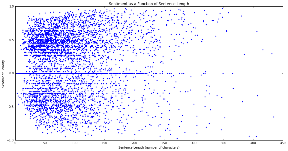

There doesn’t seem to be too much here. There is again a trend toward sentences of all length being more positive, but we already saw that in the other plots.

More to Come!

Overall, the sentiment analysis of Anne of Green Gables was a success! I am actually pleasantly suprised at how well the sentiment changes were captured over the whole novel. This is just the start of analyzing Montgomery’s writing, so please check back in to read more.